Traditional portfolio optimization (often called modern portfolio theory, or mean-variance optimization) balances expected portfolio return with expected portfolio variance. You input how opposed you are to portfolio variance (your risk tolerance), then you build a portfolio that gives you the best return given your risk tolerance.
Goals-based investing, by contrast, defines “risk” as the probability of not achieving your goal. We assume you want to minimize that risk, so that is the only portfolio objective of a goals-based investor. As you will see, variance and returns are inputs into that equation, but they are not the equation (I rant more about that here).
For the most part, goals-based optimization produces portfolios that are on the mean-variance efficient frontier, but not always. I won’t go into why that is in this post (here is why), but I will demonstrate when the two methods diverge.
Fundamentally, there are three basic steps to optimizing a goal-based portfolio:
- Determine your goal variables: time horizon, amount of wealth dedicated to the goal today, and future required wealth value.
- Develop capital market expectations for your investment universe: correlations, return expectations, and volatility.
- Run a standard optimizer with a goal-based utility function.
This post is all about how to optimize a goal based portfolio in R.
First, we need to understand the goal, what is it you want to do with the money? To keep things simple, let’s say you need $1,000 in 10 years, and you have $750 dedicated to it today. We organize this into a goal vector with the goal’s value, the required funding value ($1,000), and the time horizon (10 years). Note that the goal’s value is only relevant when optimizing your current wealth across your goals, which this post does not cover.
pool <- 750 # Total amount dedicated to this goal
goal_vector <- c(1, 1000, 10) # c(Goal value, goal funding requirement, time horizon)
Ok. Step 1 is done.
Second, we need to develop capital market expectations for our investment universe. This topic is so big numerous books have been written on it because it is a very important step. Better forecasts yield better results. Since this post isn’t about building CMEs, let’s just input something simple.
- Stocks: 9% average return with 15% volatility
- Bonds: 4.5% average return with 5% volatility
- Gamble: -1% average return with 80% volatility
- Cash: 0.5% average return with 0.01% volatility
# Asset names
assets <- c('Stocks', 'Bonds', 'Gamble', 'Cash')
# Capital Market expectations - each is a vector in order of assets
cme <- data.frame( 'Return_Forecast' = c(0.09, 0.045, -0.01, 0.005),
                   'Volatility Forecast' = c(0.15, 0.05, 0.80, 0.001) )
# Correlation matrix, in order of assets both sideways and vertically
correlations <- matrix( c(1.00, 0.10, 0.00, 0.00,
                          0.10, 1.00, 0.00, 0.00,
                          0.00, 0.00, 1.00, 0.00,
                          0.00, 0.00, 0.00, 1.00),
                        nrow = length(assets), ncol = length(assets), byrow=T )
Note the “gamble” asset–we are going to have fun with that in a minute! Step 2 is complete.
Finally, now that we have our human-based inputs, let’s proceed with the algorithm. Load our required libraries.
library(tidyverse)
library(Rsolnp) # this is the optimizer solnp()
And build the functions we will use.
# Required Functions
# This function converts the covariance table and weight vector into a
# portfolio standard deviation.
sd.f = function(weight_vector, covar_table){
  covar_vector = 0
  for(z in 1:length(weight_vector)){
    covar_vector[z] = sum(weight_vector * covar_table[,z])
  }
  return( sqrt( sum( weight_vector * covar_vector) ) )
}
# This function will return the expected portfolio return, given the
# forecasted returns and proposed portfolio weights
mean.f = function(weight_vector, return_vector){
  return( sum( weight_vector * return_vector ) )
}
# This function will return the probability of goal achievement, given
# the goal variables, allocation to the goal, expected return of the
# portfolio, and expected volatiltiy of the portfolio
phi.f = function(goal_vector, goal_allocation, pool, mean, sd){
  required_return = (goal_vector[2]/(pool * goal_allocation))^(1/goal_vector[3]) - 1

  if( goal_allocation * pool >= goal_vector[2]){

    return(1)

  } else {

    return( 1 - pnorm( required_return, mean, sd, lower.tail=TRUE ) )

  }
}
# For use in the optimization function later, this is failure probability,
# which we want to minimize.
optim_function = function(weights){

  1 - phi.f(goal_vector, allocation, pool,
            mean.f(weights, return_vector),
            sd.f(weights, covar_table) )
}
# For use in the optimization function later, this allows the portfolio
# weights to sum to 1.
constraint_function = function(weights){
  sum(weights)
}
Since we input correlations and volatilities, we need to build a covariance table. This uses the

form (covariance of asset i to j equals the correlation of i and j times the volatility of i times the volatility of j).
# Convert correlations to covariances
covariances <- matrix( nrow = length(assets), ncol = length(assets) )
for(i in 1:length(assets)){
  for(j in 1:length(assets)){
    covariances[j,i] <- cme[i,2] * cme[j,2] * correlations[i,j]
  }
}
All that is left is to do the optimization
# Optimization
return_vector <- cme$Return_Forecast
covar_table <- covariances
allocation <- 1
starting_weights <- rep(0.25, length(assets)) # start with 25% weights
result <- solnp( starting_weights, # Initialize weights
                 optim_function, # The function to minimize
                 eqfun = constraint_function, # The constraint function ( sum(weights) )
                 eqB = 1, # Constraint function must equal 1
                 LB = rep(0, length(assets)), # Lower bound of constraint, weight >= 0
                 UB = rep(1, length(assets)) ) # Upper bound of constraint, weight <= 1
# Results
optimal_weights <- data.frame( 'Assets' = assets,
                               'Optimal Weights' = round(result$pars, 2) )
The solnp function from the Rsolnp package is quite powerful. Plus, when you are running it on complicated problems, the output makes me feel like a hacker, which is always a plus!
And we find that our optimal weights are 31% stocks, 69% bonds.
So What’s Different About Goals-Based Investing?
Now that you’ve got the basics of goals-based portfolio optimization, we may ask what is so different about GBI? Well, let’s find out!
To illustrate, let’s build allocations for various levels of starting wealth.
pool_seq <- seq(50, 1000, 50)
And empty lists to hold the various allocation results
# Empty lists of allocation to hold results
stock_allocation <- 0
bond_allocation <- 0
gamble_allocation <- 0
cash_allocation <- 0
Then iterate through each starting wealth value and determine the optimal investment allocation (this code assumes you’ve run the code in the previous section).
# Loop through each level of starting wealth to determine optimal allocation
for(i in 1:length(pool_seq)){
  pool <- pool_seq[i]
  result <- solnp( starting_weights,
                   optim_function,
                   eqfun = constraint_function,
                   eqB = 1,
                   LB = rep(0, length(assets)),
                   UB = rep(1, length(assets)) )

  # Store results for this iteration
  stock_allocation[i] <- result$pars[1] %>% round(digits = 2)
  bond_allocation[i] <- result$pars[2] %>% round(digits = 2)
  gamble_allocation[i] <- result$pars[3] %>% round(digits = 2)
  cash_allocation[i] <- result$pars[4] %>% round(digits = 2)
}
Since I am using ggplot, I’ll now need to store the results in a long form data frame.
seq_results <- data.frame( 'Weight' = c(stock_allocation,
                                        bond_allocation,
                                        gamble_allocation,
                                        cash_allocation ),

                           'Asset' = c( rep('Stock', length(stock_allocation)),
                                        rep('Bond', length(bond_allocation)),
                                        rep('Gamble', length(gamble_allocation)),
                                        rep('Cash', length(cash_allocation))),

                           'Wealth' = rep(pool_seq, length(assets)) )
And, finally, visualize the results.
ggplot( seq_results, aes(x = Wealth, y = Weight, fill = Asset))+
  geom_area( linetype=1, size=0.5, color='black')+
  xlab('Initial Wealth')+
  ylab('Investment Weight')+
  labs(fill = 'Asset',
       title = 'Optimal Allocation for Various Levels of Starting Wealth',
       subtitle = 'Goals-based optimization')
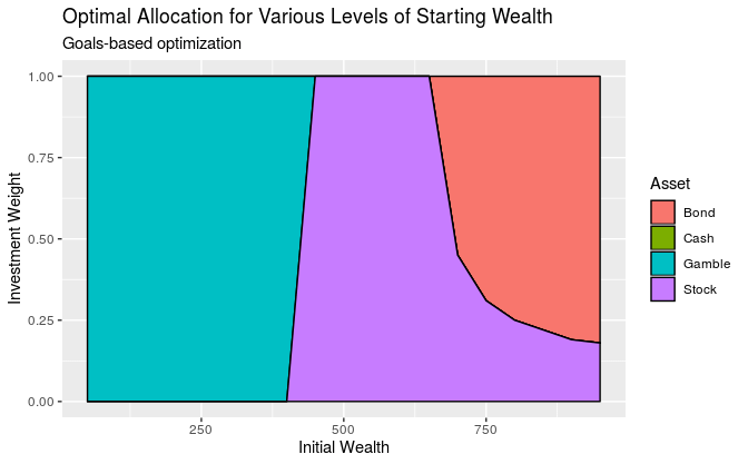
As you can see, goals-based portfolios will lean on high-variance, low return investments when your starting wealth is small enough. Technically speaking, GBI portfolios begin allocating to lottery-like investments whenever the return required to hit the goal is greater than the return offered by the mean-variance efficient frontier. In traditional mean-variance optimization, the optimizer will maintain exposure to the endpoint of the frontier, or 100% stock allocation, in our example.
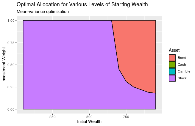
As a comparison, here is the mean-variance optimizer result. As you can see, the “gamble” asset is eliminated from consideration.
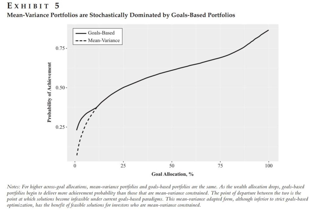
Because of this, goal-based portfolios yield higher probabilities of goal achievement than mean-variance portfolios (mean-variance portfolios are stochastically dominated by goals-based portfolios). This was Exhibit 5 in my recent paper on this subject.
For all of these reasons (and more), if you have goals to achieve then you should be using goals-based portfolio theory. I hope this post helped you understand how to implement the basic framework!
Goals-based portfolio theory is also concerned with how you allocate your wealth across your goals, which I have not covered in this post, but I will cover that in a later discussion.
Keywords: goals-based investing, goal based investing, investing, portfolio theory, portfolio optimization.